If you’ve not heard of them, autostereograms are simply a form of stereogram (e.g. a stereo image pair) made for viewing without special equipment (see, for example, Wikipedia for more detailed info). They became amazingly popular in the 1990s mostly because of the equally popular Magic Eye books. And while they will never rival the quality of modern 3D imagery they can still be incredibly fun – assuming you’re willing to put the eye-popping effort into managing to view them. So I decided I ought to add them to the Python 3 Photos3D library which you can find at the Parth3D Github repository.
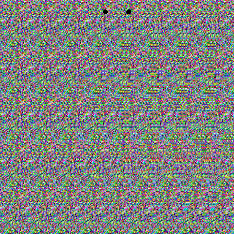
I’ve put an example autostereogram below. If you don’t know what you’re doing just try to relax your focus until the two dots at the top merge and you see three. At that point you should see a 3D image appear, in this case of an anchor. There are a number of different types of these images and this one is a random dot stereogram. That just means the background image is made up of random dots which, in the Photos3D library code, can be multi-colour or monochrome. And the library code also allows use of tiles made from real images, as you’ll see soon. You’ll hopefully notice that the pattern is a repeating tile in a grid which, together with a depthmap image, is an essential aspect of our code.
If you’re not interested in the Python 3 coding aspect feel free to jump down to the implementation. Otherwise you will surely want to know how we create a stereogram in Python code? Well, it’s actually incredibly easy once you know a few things. To make those things clearer I’ve put a diagram below. The main thing to note is that we will mostly be working on the output image – that is, we will be both reading pixel colours, and writing them, in the output file. That may sound odd, but it’s simply because the process involves changing the pattern width, along each scan line, to represent changes in depthmap values. That may sound a bit (actually very) complicated, but hopefully the code will make it clearer (or see this blog post which I found very clear on the theory).
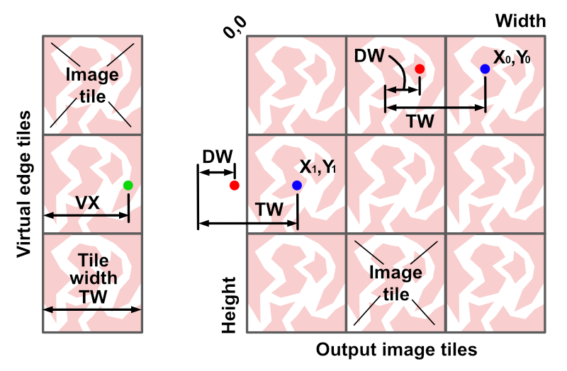
We can create the output image by looping over X and Y values for the width and height. If we look closely at the diagram above, we can see a pixel at X0, Y0. To work out the colour we use a pixel to the left, where we have already written a colour. The X coordinate is adjusted negatively (left) by one tile image width, and positively (right) by a small amount determined from the X0, Y0 position in a corresponding depth map. But you’ll also notice that, for the pixel at X1, Y1, the process leads to a negative X value which will cause our code to bomb out with an index out of bounds error. So for that situation, which should only occur at lower X values, we read the position VX from the tile image instead: VX = TW – (X – TW + DW) which in maths terms can obviously be simplified.
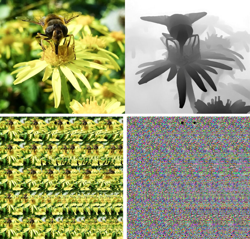
If you download the code from the Parth3D Github repository you can run the example on your commandline something like ‘python autostereo.py’. It uses the RGB-D image of a bee on a flower, which has the colour image on the left and the monochrome depthmap (made by the excellent DepthMaker Android app) on the right. Using that image a stereogram will be created and displayed. You can change between random dot and image pattern for the tile by commenting, and uncommenting, some lines that are discussed in the code source file. You can see the RGB-D image, together with both of those outputs, in the image below.
If you read the autostereo.py file you can see how we load the depthmap and make the tile image (which doesn’t have to be square, by the way), as well as how we call the library code to make the output image. But all of the real magic happens in the library’s depthmaps.py module which has a new function called depth_to_autostereo. It’s actually very short so I’ve included it in full below. It requires an image tile (astile), the number of tiles needed in the X and Y directions (numx and numy) and a numpy array of depth values between 0 and 255 (depths). It will calculate disparity values for you automatically, but if you’re keen you can look at depthmaps.py and create your own disparity values (dispvect). Also, we will add the dots at the top of the stereogram by default (helpers).
def depth_to_autostereo(astile, numx, numy, depths, dispvect=None, helpers=True):
    tile = image_copy(astile)
    tw, th = tile.size
    if dispvect == None:
        dispvect = create_linear_disparity_vector(int(tw/2), 0, doreverse=True)
        pass
    edge = tile_image(tile, 1, numy)
    imgin = tile_image(tile, numx, numy)
    wid = numx * tw
    hgt = numy * th
    imgme = __blank_image__(wid, hgt, col=(0, 0, 0))
    inpix = imgin.load()
    mepix = imgme.load()
    edpix = edge.load()
    col = inpix[0, 0]
    for y in range(0, hgt):
        for x in range(0, wid):
            dep = int(depths[y, x])
            lrdisp = int(dispvect[dep])
            dx = x + lrdisp - tw
            if dx < 0:
                col = edpix[tw + dx, y]
            elif dx < wid:
                col = mepix[dx, y]
            mepix[x, y] = col
    if helpers:
        add_helpers(imgme, 50, dispvect[-1], 10, col=(0, 0, 0))
    return imgme
Hopefully the code is fairly clear. The for loops let us iterate over the output image pixels. For each pixel a revised X value is calculated and the offset pixel colour copied. I coded it so the left edge negative X values are converted to coordinates in an image one tile wide by numy high. That just makes the coding a bit easier – you could use the tile image and use a revised Y value, based on using the modulus of dividing Y by the tile height (assuming you’re that kind of adventurous type). Otherwise, the code is just a simple use of the Python Pillow library to load image pixels and set their colours. I think the real expertise comes in deciding on the image and tile dimensions, as well as the maximum disparity. In terms of the latter I’ve found half the tile width is a sensible maximum, as the image starts to break down quite significantly at higher values – but why not give that a go yourself and see what you think.
And that’s it – we can now dazzle our family and friends with some retro 1990s cool! Well, perhaps just the ones who can look at images while crossing their eyes, and looking like their eyeballs will pop out, anyway 🙂


