Taking 360-degree photos is a lot of fun, but it’s very difficult to take stereoscopic 3D VR photos that look good all around. So I decided to have a go at making textured spheres to let me render images and videos in Blender, using its’ 3D camera. The easiest way to do that is to use a an AI-generated depthmap and, having used Looking Glass Blocks previously, I decided to see how it would cope with 18-megapixel equirectangular photos generated by an Insta360 camera. As it turned out, Blocks did a pretty good job of it, as the VR360 photo below, from lovely Parc Howard in Llanelli, shows.

Creating the textured sphere is done using Python 3 with some fairly simple code. That code comes in two files, which you can find, and of course download, on the Parth3D Github repo. One of them is called objfile.py and, while I won’t cover it here, you can delve into it to see how the code saves 3D geometry data to OBJ files for importing into Blender. The other file, called simple_texball.py, holds the main code we’re interested in here – it creates the spherical 3D geometry and the texture coordinate data, plus it saves the Wavefront OBJ and MTL files.
If you’re not interested in coding you can just use Python at the commandline to run the code (e.g. run python simple_texball.py and it’ll produce the OBJ and MTL files for you), then import the generated example OBJ file into Blender and play. But for everyone else, I’ll cover how it works below. If you open simple_texball.py in your favourite IDE, or on the Github repo webpage, you’ll see it includes a couple of library imports. The math library is just there for calculating the 3D positions of vertices, and the Pillow image library is used for reading depth data from the monochrome depthmap image.
import math
from PIL import Image
Next, we need a way to generate the vertices and faces of a sphere. That’s done using the sphere_with_seam function below. It’s quite simple if you look at it in sections. It starts by calculating the positions for a semi-circular arc in two dimensions, before using those data to calculate the 3D positions around the sphere. It’s basically a solid-of-revolution algorithm, but note that the angle change between vertices around the equator is designed so the last vertex is at the same position as the first, for each row – basically that’s so we end up with an unclosed seam as that’s how we ensure we can texture a sphere, and save it in an OBJ file, with the texture image going all the way around.
def sphere_with_seam(latincs, longincs):
    # Create half circle cross section
    xs = []
    xs.append([0, 1])
    ainc = math.pi / (latincs - 1)
    for c in range(1, latincs - 1):
        x = math.sin(c * ainc)
        y = math.cos(c * ainc)
        xs.append([x, y])
    xs.append([0, -1])
    vertices = []
    faces = []
    numpts = latincs
    # Create vertices
    for c in range(0, numpts):
        y = xs[c][0]
        z = xs[c][1]
        if c == 0 or c == (numpts - 1):
            vertices.append([0, 0, z])
        else:
            for xincs in range(0, longincs):
                pangle = (xincs / (longincs - 1)) * (2 * math.pi)
                vertices.append([y * math.sin(pangle), y * math.cos(pangle), z])
    ev = len(vertices) - 1
    # Create faces
    for c in range(0, numpts):
        for xincs in range(0, longincs - 1):
            if c==0:
                tl = 0
                bl = ((c + 1) * longincs) + xincs - longincs + 1
                if xincs < (longincs - 1):
                    br = ((c + 1) * longincs) + xincs + 1 - longincs + 1
                else:
                    br = ((c + 1) * longincs) + xincs + 1 - longincs + 1 - longincs
                faces.append([tl, br, bl])
            elif c == (numpts - 1):
                tl = (ev - longincs) + xincs
                if xincs < (longincs - 1):
                    tr = tl + 1
                else:
                    tr = ev - longincs
                bl = ev
                faces.append([tl, tr, bl])
            elif c < (numpts - 2):
                tl = (c * longincs) + xincs - longincs + 1
                bl = ((c + 1) * longincs) + xincs - longincs + 1
                if xincs < (longincs - 1):
                    tr = (c * longincs) + xincs + 1 - longincs + 1
                    br = ((c + 1) * longincs) + xincs + 1 - longincs + 1
                faces.append([tl, tr, br, bl])
    return [vertices, faces]
The last part of the function calculates which vertices make up each individual face. As quads work much better in Blender rendering, compared to triangles, especially when using smooth shading, we specify four vertices per face. Finally the function returns two lists: one of all the vertices and one for all the quad faces. And so you can see what the function produces, below is an image of a sphere created with it, with our soon to be added texture image drawn on it.

For the texturing we’ll need a way to load images. We won’t actually need to load the texture image, but we will need to read pixel values from the depthmap image. The load_image function below does just that, also allowing us to specifiy a maximum image width: if the loaded image is wider it will be resized while respecting the aspect ratio. At the end we also convert the image to an ‘RGB’ format. That’s very important for one reason: monochrome images can have one or three buytes per pixel. So converting the image to three bytes per pixel saves us having to write complex code later, to cover both scenarios.
def load_image(fn, maxwid=None):
    im = Image.open(fn)
    if maxwid != None:
        w, h = im.size
        print("Original image size is " + str(w) + " x " + str(h))
        if w > maxwid:
            asp = w / h
            nh = int(maxwid / asp)
            #im = im.resize((maxwid, nh), Image.Resampling.LANCZOS)
            im = im.resize((maxwid, nh))
            print("Image resized to " + str(maxwid) + " x " + str(nh))
    im = im.convert('RGB')
    return im
As we can now load images we can also use them to calculate depth values from the brightness of individual pixels. With the Looking Glass Blocks map black is further away and white is closer up, so our code will assume that (if you have problems make a negative image of the map in an image editor). The adjust_sphere_depth function below does that by loading a big list of all the pixels and using the red-channel value, between 0 and 255, to interpolate between our minimum and maximum radii. It simply adjusts the depth by multiplying the x, y and z parts of the vertex by the calculated depth – that’s possible because we made our sphere have a radius of one, which is essentially a normalised vector (i.e. the vector has unit length).
def adjust_sphere_depth(verts, dim, wrad, brad):
    nverts = []
    dw, dh = dm.size
    dpix = dim.load()
    # Calculate depth for top / zenith vertex
    col = dpix[int(dw / 2), 0]
    din = 1 - (float(col[0]) / 256)
    dep = (din * (brad - wrad)) + wrad
    nverts.append([verts[0][0] * dep, verts[0][1] * dep, verts[0][2] * dep])
    # Calculate depth for all vertices between top and bottom ones
    for y in range(1, dh - 1):
        for x in range(0, dw):
            col = dpix[(dw - 1) - x, y]
            din = 1 - (float(col[0]) / 256)
            dep = (din * (brad - wrad)) + wrad
            ind = 1 + ((y - 1) * dw) + x
            nverts.append([verts[ind][0] * dep, verts[ind][1] * dep, verts[ind][2] * dep])
    # Calculate depth for bottom / nadir vertex
    col = dpix[int(dw / 2), dh - 1]
    din = 1 - (float(col[0]) / 256)
    dep = (din * (brad - wrad)) + wrad
    nverts.append([verts[-1][0] * dep, verts[-1][1] * dep, verts[-1][2] * dep])
    # Now smooth the seam by averaging
    for y in range(1, dh - 1):
        ind0 = 1 + ((y - 1) * dw)
        ind1 = 1 + ((y - 1) * dw) + (dw - 1)
        vec0 = nverts[ind0]
        vec1 = nverts[ind1]
        nverts[ind0] = [(vec0[0] + vec1[0]) /2, (vec0[1] + vec1[1]) /2, (vec0[2] + vec1[2]) /2]
        nverts[ind1] = nverts[ind0]
    return nverts
Hopefully you’ll have noticed that the above code also smoothed the seam vertices by averaging them. That’s necessary because the AI making the depthmap doesn’t know that the left and right sides of the image are actually the same place: if you notice big unwanted steps at the seam you could adjust the code to average using more vertices. And next we need to calculate the texture coordinates, which are basically similar to x and y coordinates for the texture image, but run from 0 to 1 (i.e. zero to 100% of the width or height). The function below, called get_sphere_texture_coords, does that for us. It produces a list of texture coordinates with one for each of the vertices. It’s quite simple as all it needs do is interpolate between 0 and 1 based on the number of vertices per row.
def get_sphere_texture_coords(imw, imh):
    tcs = []
    tcs.append([0.5, 1])
    for y in range(1, imh - 1):
        ty = 1 - (y / (imh - 1))
        for x in range(0, imw):
            tx = 1 - (x / (imw - 1))
            tcs.append([tx, ty])
    tcs.append([0.5, 0])
    return tcs
And that’s all the functions we need. All that we need do now is run them from the code below, as described earlier. You’ll be able to scale the generated sphere in Blender later if you like, but I’d advise thinking carefully about the start (srad) and end (erad) radii values carefully and adjusting them as needed. Also, we want a good quality texture image, but only a simpler representation of the 3D geometry. So I made the code resize the loaded depthmap image to around 5% of it’s original width – I found that a good tradeoff between enormous OBJ files and 3D render quality, but you’ll need to play with it to find what’s best for you. And, if you just want a textured sphere, ignoring the depthmap, you can easily do that by commenting out the adjust_sphere_depth line.
if __name__ == '__main__':
    import objfile as obj
    srad = 2
    erad = 15
    print("Simple Textured Ball to OBJ test.")
    dm = load_image("simpletexball_depth.jpg", maxwid=304) # 5% of RGB width
    dw, dh = dm.size
    verts, tris = sphere_with_seam(dh, dw)
    verts = adjust_sphere_depth(verts, dm, srad, erad)
    texcoords = get_sphere_texture_coords(dw, dh)
    obj.write_obj_file("simpletexball", "simpletexball", verts, tris, None, texcoords, swapyz=True)
    obj.write_mtl_file("simpletexball", "simpletexball_rgb.jpg")
    print("Finished.")
The OBJ file generated when we run the above code, with the images provided on Github, can now be imported into Blender using the Wavefront OBJ option. You can choose which axes face up and forward in the import dialog, as often OBJ files have up along the y axis, rather than the z axis as is more usual in Blender. However, you’ll notice the OBJ library has an option called swapyz, which I set to true. That means that if you use the code as shown above then the imported model in Blender should be correctly orientated, as shown in the screen grab below.

If you now zoom into the sphere in Blender you can see the view from the inside, as shown below, which is what we’re mostly interested in as a render backdrop. You may notice sharp changes in depth look a bit blocky, but that’s OK as we can select the sphere, right click on it and select the smooth shading option. That should make our depth-adjusted sphere look much more natural in our renders. However, for the best quality renders you’ll likely want to play with the size of the depthmap used to generate the sphere: I used 5% of the width, but you may want a bit more to increase the number of vertices (albeit with a corresponding increase in file size and memory requirements).

If you look at the image above you may also see a little quirk of my method. The AI that created the depthmap didn’t know the bottom of the image is the bottom of a sphere. So the points around the zenith (top vertex) and nadir (bottom vertex) can poke up a little. If that’s noticable in your renders you can easily change the camera clipping distance, or flatten the offending vertices. And, of course, the depth affect really needs to be viewed from the centre of the sphere (see the grass and bushes in the above image for an example of what happens with the camera away from centre), rather limiting camera positions. However, even with some minor problems, depthmap-adjusted textured spheres are, in my humble opinion, an extra bit of fun when playing with 3D rendering 🙂


