A while back I was looking at some anaglyph photos and pondering how the two views converge to form a 3D image. So I wrote some simple Python 3 code to explore that and decided to share it here in case others find it useful too. And it turns out to be quite easy to plot disparity: it can be calculated as the difference in angles, between where we’re looking and where another point in space is, between the left and right views. Clear as mud! So while I’m sure my explanations below might be a little difficult to understand at first, I hope the Python code on the Parth3D Github repo, together with the diagram below, will be a much more enjoyable way to explore the concepts.
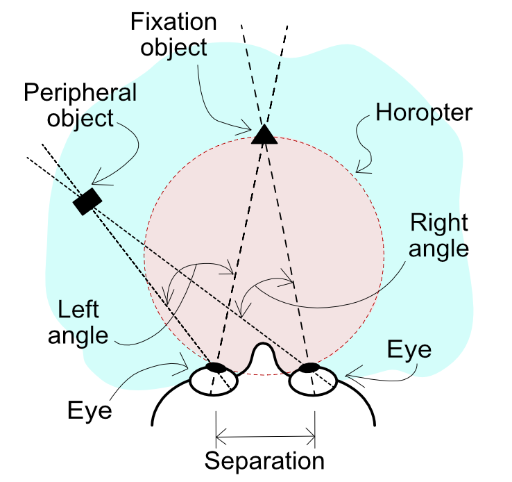
As the diagram shows, we’re assuming here that we’re looking at a point of fixation (i.e. what we’re looking at) straight ahead of us. That point is where our left and right views converge, so that fixation object will have no disparity between the left and right views (i.e. they’re in the same place on the retina or image sensor). If another point in our field of view is then considered, such as an object on the periphery, the left and right vectors to it don’t necessarily lie at the same angles from left and right fixation vectors. So the difference in those angles basically defines the degree of disparity our brains perceive. Because of that it’s relatively easy to write some Python 3 code to plot disparity looking down on our heads (or a camera if you prefer).
I won’t put the whole of the code here because you can download it from the Parth3D Github repo. But I’ve put below the code for calculating disparity as it’s the most important bit. All it does is iterate over each pixel in an image xnum pixels wide by ynum pixels high, as long as it is within the field of view (degfov in degrees) and minimum distance away (mindist in metres). Using the eye/view separation (sep in metres) and convergence (convdist in metres) distances it then works out the left and right fixation vector angles, and from the x and y corrdinates it calculates the pixels’ angles too. It then calculates how many degrees difference there are between the left and right angular differences, and saves that to a list which the rest of the code makes a lovely coloured image from.
def calcdisparity(degfov, sep, convdist, mindist, xnum=501, ynum=500, scl=1):
wid = xnum
if wid % 2 == 0:
wid = wid + 1
hgt = ynum
eyerot = math.atan((sep / 2) / convdist)
fov = math.radians(degfov)
disparity = []
for cy in range(0, hgt):
ldisp = []
for cx in range(0, wid):
x = (cx - int(wid / 2)) * scl
y = (cy * scl) + (scl / 2)
dist = math.sqrt(x * x + y * y)
lang = (math.atan((x + sep / 2) / y) + 1000) - (eyerot + 1000)
rang = (math.atan((x - sep / 2) / y) + 1000) - (-eyerot + 1000)
if abs(lang) <= (fov/2) and abs(rang) <= (fov/2) and dist >= mindist:
dang = (lang + 1000) - (rang + 1000)
else:
dang = None
ldisp.append([dang, lang, rang])
disparity.append(ldisp)
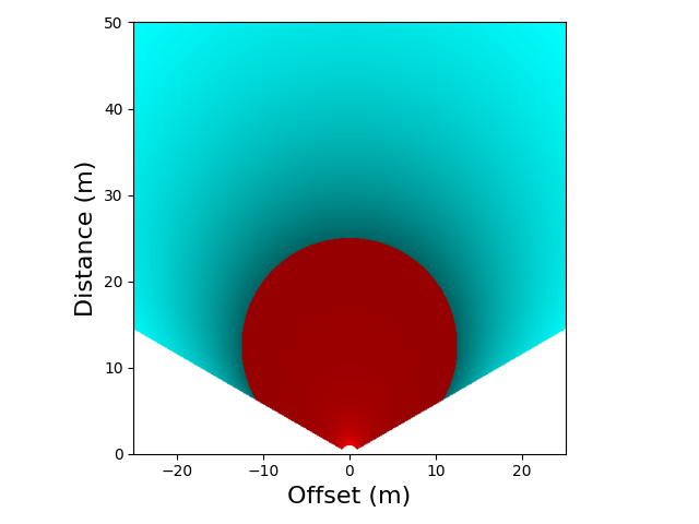
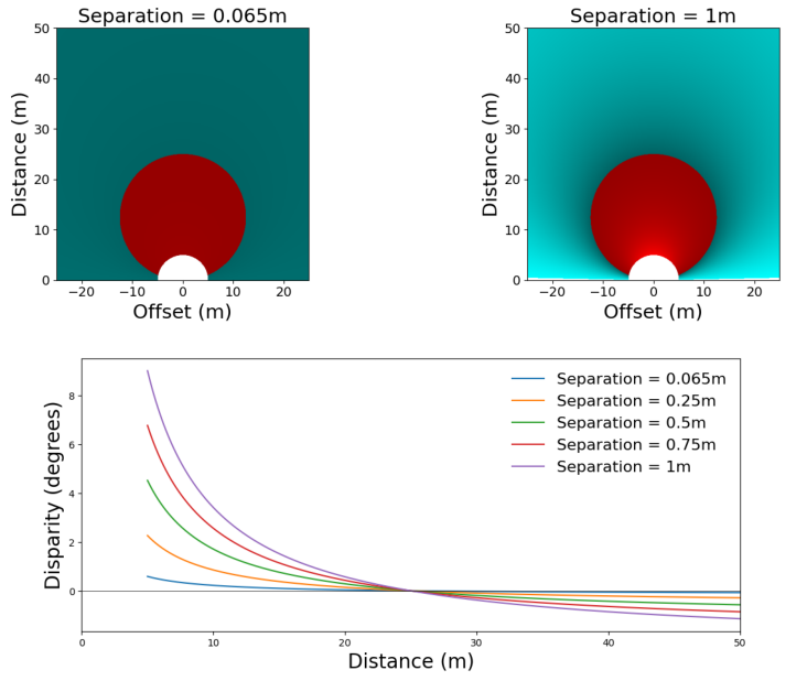
return disparityIf you run the example on the Github repo you’ll get a plot like the one below. As with all the following examples I’ve used a scale of 0.1m per pixel, to give a plan around 50m per side with the default of 501 for xnum and 500 for ynum. The eye separation in the plot is 0.065m, which is a common value for adult humans, and the eyes are converging at a distance, straight ahead, of 25m. What’s interesting is that the red area is ‘normal’ divergence and it reduces up to zero at a circle through the fixation point. It turns out that circle is called the horopter (see earlier diagram and Wikipedia) and past it (the cyan area) disparity increases but in a negative way (e.g. for an anaglyph cyan on the left would change to red on the left). So we can see how much disparity we can expect for an object placed anywhere in our field of view.
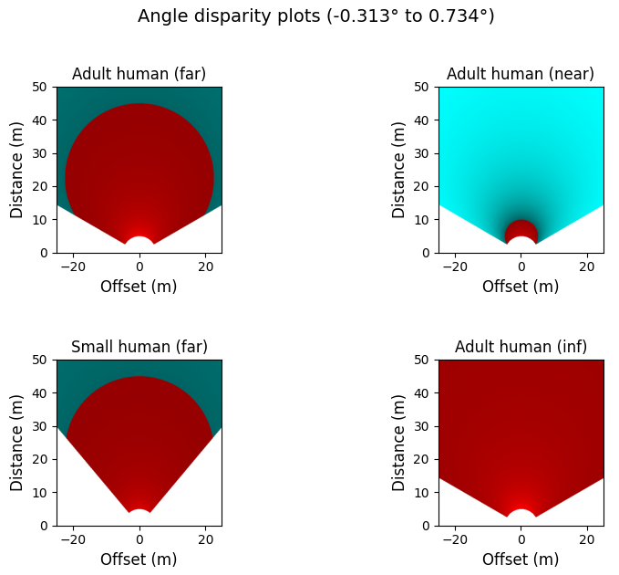
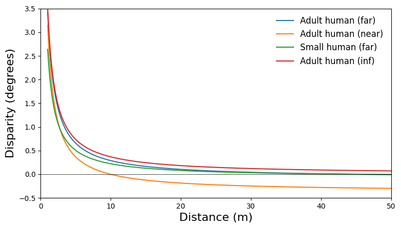
So hopefully the Python example code isn’t too difficult to understand, and the main thing is to understand the main variables we covered above for the code to calculate disparity. If so, that means we can play about with the variables to explore how the horopter and disparity work. I decided to try a few examples out, the parameters for which I’ve put in the table below.
| Field of view | Separation (m) | Convergence (m) | Start (m) | |
| Adult human (far) | 120 | 0.065 | 45 | 5 |
| Adult human (near) | 120 | 0.065 | 10 | 5 |
| Small human (far) | 80 | 0.05 | 45 | 5 |
| Adult human (inf) | 120 | 0.065 | 1000 | 5 |
They’re mostly based around looking near (10m) and far (45m), as well as looking pretty much into infinity (1000m). I also tried the near convergence with a smaller separation and field of view, to see how much difference being a child makes. The plots for them are below and I learned a lot from them. Basically, as expected, the horopter shrinks and grows with the convergence distance to our point of fixation. Plus the difference between a child and adult isn’t that much, mainly it’s about slight tunnel vision when younger. And, of course, the horopter disappears when we look toward infinity, because the views from our eyes don’t converge. And convergence inside the horopter is much greater than beyond it, although for looking close up I expect that a lot of what’s close and high-disparity is also out of focus.
To make that clearer I’ve also put a graph below showing the disparity, in degrees, for the above plots, along the line directly up the middle of the plots. Hopefully they make the above plots clearer, and I think they’re quite useful in showing that the convergence distance has a big impact on the amount of disparity we perceive, with bigger disparity either side of the horopter when viewing closer. And that seems very true too for ‘reverse / negative’ disparity after the horopter. And, again, please remember that the large close-up disparities would likely be at distances where any object there would be out of focus anyway.
Finally, I also thought it would be quite interesting to see how much we can change disparity by changing the separation, like when we take two photos in smartphone apps and turn them into stereo views. The results of that are below, for separations up to a metre. As I’m sure you expected, increases in separation amplify the disparity within and outside the horopter. However, as you’ll probably have guessed from the above, it has very little effect on the horopter, just widening it slightly. Of course that will vary a lot too with convergence distance, which you can explore through the Python code if you wish.
And while that’s just a brief introduction of what we can find out using the Python code, I hope you agree it’s a good start for more in-depth investigations on disparity, horopters and stereo vision in general. I hope you found it useful 🙂


