
The exciting thing about coding is we can create 3D models parametrically: that is, we can change parameters and our code will update the 3D model accordingly. For many purposes that’s great, but of course sometimes we also want to create 3D models using a 2.5D process. By that I mean that we design a cross section for a part, and then extrude it to the finished 3D shape. Of course, we can do that in code, but often we will use CAD software to give us the greatest flexibility when defining the cross-section. And CAD will almost ubiquitously be able to import DXF files, making it a very useful interchange format between code and 3D model generation.
For that reason, ezDXF is a very useful Python library, allowing us to generate AutoCAD DXF files straight from our code. It’s very easy to use and you can easily generate lines from simple lists (a.k.a. arrays) of X and Y vertices. And obviously OpenSCAD is one of the main ways makers like to generate 3D content from DXF files. In fact, OpenSCAD makes the process almost trivial, and FreeCAD includes an OpenSCAD workbench if you prefer that software. So I decided to write some code as a simple illustration of how to make a 3D part in OpenSCAD using ezDXF and Python 3. And given that I like mobile coding, all of the code is written and tested on Android too, so I’ll cover the best method for use in PyDroid3 and ScorchCAD as well.
The first thing you need to do is use pip to add the ezDXF library into your Python 3 installation: click here for the PyPi page that tells you how. If you’re using PyDroid3 on your phone or tablet, just type ‘ezdxf’ into the install box in the pip page and it should simply install it. The only other prerequisites are matplotlib and numpy, but I’ll assume you know enough about Python to install them and run the code from an IDE or the command line. Then, to test ezDXF we’ll need a list of 2D vertices for exporting to DXF. I decided a simple cog design would be a good example, so I wrote the Python3 code below. So if you want to have a go, simply copy and paste the code into your Python editor.
import math
opts = [] # Outer points list
ipts = [] # Inner points list
orad = 10 # Outer radius
inset = 1.5 # Inset for cog teeth
irad = 2 # Inner radius
teeth = 25 # Number of teeth on cog
numpts = teeth * 2 # Number of points around cog
for c in range(0, numpts):
ang = (2 * math.pi) * (c / numpts)
crad = orad
if (c % 2) != 0:
crad = orad - inset
opts.append([crad*math.sin(ang), crad*math.cos(ang)])
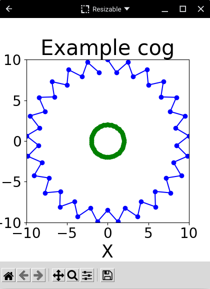
ipts.append([irad*math.sin(ang), irad*math.cos(ang)])If you’re a newbie coder that may seem a bit complicated. But look closely, the code is just calculating the X and Y coordinates around a circle at an increasing angle. And for every other outer point it’s reducing the radius a small amount, creating ‘teeth’ that form a cog shape. I’ve used 50 points around both, which is equivalent to using $fn = 50; in OpenSCAD when creating a cylinder. So now we have a list of 2D vertices in the format [ [x0, y0], [x1, y1], … [xN, yN] ] where N is the index of the last vertex. Obviously you’ll want to see what the 2D sections look like: to do that, add the code below to the end of your Python file.
import matplotlib.pyplot as plt
import numpy as np
xy=np.array(opts)
plt.plot(xy[:,0],xy[:,1], linestyle='solid', marker='o', color='blue')
xy=np.array(ipts)
plt.plot(xy[:,0],xy[:,1], linestyle='solid', marker='o', color="green")
plt.axis('square')
plt.xlim(-10, 10)
plt.ylim(-10, 10)
plt.title("Example cog",fontsize=30)
plt.xlabel('X',fontsize=25)
plt.ylabel('Y',fontsize=25)
plt.tick_params(labelsize=20)
plt.xticks([-10, -5, 0, 5, 10])
plt.yticks([-10, -5, 0, 5, 10])
plt.show()
That’s basic matplotlib code for plotting lists of 2D points using numpy arrays, so I won’t spend time describing it too much here. Basically it should output a graph window that looks like the one below. Note that my screenshot is from PyDroid3 on my Chromebook, but it should work pretty much the same on any device where you run Python 3 code. Now, there’s one very important thing to note about the plot: it isn’t closed. By that I mean that, if you look at the top of the plot, you’ll notice there’s a gap between the last and first vertices. You’ll discover why very soon.
Now we have a section through our cog design, how do we export it into the DXF file? Well, firstly let me mention that there are two main ways we can go about it. The first way is to iterate through our vertices list and get ezDXF to draw a line for each vertex to the next one along. And actually that will work fine with OpenSCAD on a PC. However, if you’re using the ScorchCAD Android app (or something similar) it won’t, simple as that. So that’s a good reason to avoid the line method, but there’s another one: suppose you want to edit the DXF file in CAD, in which case something as simple as offsetting your section could mean selection tens, hundred, or even thousands of individual line elements. Sounds scary right? Well, maybe not quite scary, but definitely rather annoying.
That’s why CAD software packages have polyline entities. If you’re not familiar with CAD, polylines let us do things like defining a path along a set of interconnected vertices. You can do some cool stuff with them, including things like adding curved regions. But for our example we’ll just use them to group all of our lines into a single entity for each section. That will have the added benefit that you can use the code with apps like ScorchCAD, which as an avid mobile coder I think is great. Fortunately ezDXF supports the common LWPOLYLINE entity so we’ll use that. And it even allows us to flag the polyline as a closed element: hence we left a gap between our first and last vertices earlier. So, without further ado, here’s the code you need to add to the end of your editor to generate the DXF file.
import ezdxf
doc = ezdxf.new('R2010')
msp = doc.modelspace()
lwp = msp.add_lwpolyline(opts, dxfattribs={'layer': 'outer'})
lwp.closed = True
lwp = msp.add_lwpolyline(ipts, dxfattribs={'layer': 'inner'})
lwp.closed = True
doc.saveas('ezdxftest.dxf')
Now you may have been expecting something more complicated. After all, we’re exporting a digital representation of some complex vertex lists. But no, it’s actually very simple to export our section lists to a DXF file. However, that’s just because we’re only exporting straight line elements to the polyline entity: it’ll get more complicated if you start adding more complex elements to the polyline. For our purposes though, once you’ve run the code above you should have a file called ezdxftest.dxf in the same folder your Python file lives in. If you want, have a look at it in a text editor. It’ll look rather unreadable (unless you’re a DXF guru) but it is plain text. You can ignore the dxfattribs bits for the moment, we’ll only need it later.
So, armed with our shiny new DXF file, let’s create a 3D model from it. I’ll start with using OpenSCAD on a PC, before showing how to do it in ScorchCAD on an Android device. So, open up OpenSCAD and create a new file in the same folder as your Python and DXF files. Obviously you could create a new folder for OpenSCAD and copy the DXF file there if you prefer, but I’m keeping it simple. Now, add the following code to the OpenSCAD window and save the file.
  linear_extrude(height = 1.5, center = true, convexity = 10)
    import (file = "ezdxftest.dxf");
The code is quite simple really, and hopefully it’ll make sense even if you’re a beginner to OpenSCAD. The import line should be self explanatory, as basically we’re importing the DXF file (although it may not be obvious that this is a 2D import as the DXF file only has two dimensions). And then we’re linearly extruding the imported data, giving it a height of 1.5 (maybe mm, or inches, or whatever dimension unit you prefer). When you saved the code you’ll have noticed OpenSCAD generated a 3D preview of the extruded cog.
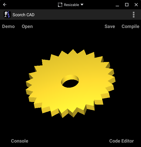
Now, if you want to do this in ScorchCAD, on your Android phone, tablet, or Chromebook, there’s an extra step. Basically, you can use the same code we used for OpenSCAD, but you need to move the DXF file to the root of your phone files, in an Android file explorer. That may be called ‘Home’, or sometimes even ‘/Storage/emulated/0’. I don’t know why, but ScorchCAD only finds DXF files when you put them there. If you then compile the file in ScorchCAD you should see something like the screenshot below. In my opinion this is very cool as it means we can do some quite complicated 3D parametric modelling wherever we are, using just our Android device!
You may have noticed that OpenSCAD (and similarly ScorchCAD) made a hole out of our inner point list. And it did it without us having to write a single line of solid constructive geometry operations. However, what if we didn’t want a hole. Maybe we really wanted the inner points list to be a shaft for our cog, in which case OpenSCAD generating a hole would be quite annoying. Well, that’s why I said I’d come back to the dxfattribs parts of the Python code later, and what better time than now?
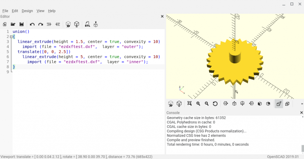
In case you don’t know, CAD, and hence DXF files, allows us to organise our entities (lines, circles, polylines, etc.) into layers. And OpenSCAD lets us import only specific layers from DXF files. Put those things together and you can see we can write OpenSCAD code to create our cog with a shaft. I’ve put the code to do that below, which you just need to paste into the OpenSCAD editor, replacing the previous code.
union()
{
  linear_extrude(height = 1.5, center = true, convexity = 10)
    import (file = "ezdxftest.dxf",  layer = "outer");
  translate([0, 0, 2.5])
    linear_extrude(height = 5, center = true, convexity = 10)
      import (file = "ezdxftest.dxf",  layer = "inner");
}
Basically, the new code imports and extrudes the layers called ‘inner’ and ‘outer’ seperately. If you’re not sure where the layer names came from look at your Python code: the dxfattribs we included in our polyline generation placed the polylines in layers with those names. We did that so we can select layers individually in OpenSCAD, and it also makes the DXF file easier to use in CAD software. And when you run the new OpenSCAD code you should see something like the screenshot below: basically our cog with a lovely shaft fused onto it.
If you’re interested in mobile 3D design you’ll be happy to know that the amended code works just as well on Android in the ScorchCAD app. And you may also like to know that all of the code is available at Github for you to download: click here to go to the Parth3D repo page. So the only thing left for me to say is that I hope you find this post useful as a way to easily create 3D models, using a 2.5D process, from 2D section data generated using ezDXF in Python 3 🙂


